Shiny apps in R

Brief introduction to Shiny

• Parts of a Shiny app
• When to use a Shiny app
• When not to use a Shiny app
  • Alternatives: Rmarkdown/Quarto, Jupyter notebooks can do R, R script and output figures

Step-by-step script to Shiny app

• Walk through the process of starting with an R script and then ending with a Shiny app

Selecting a dataset

Let’s use a fun dataset. This post produced the GIF below in R showing monarch butterfly migrations.

• https://medium.com/@jakeamahr/using-rgbif-to-visualize-annual-monarch-butterfly-migrations-f34a335b77f1

  

  Monarch Butterfly Migrations

• We won’t replicate this (you can follow the link if you would like to do that), but we can use the same data source.

The Global Biodiversity Information Facility (GBIF) is a free an open access database with a lot of information that can be mined about all different species of organisms.

• https://www.gbif.org/

• There is an R package that makes it easy to access this data:

  • https://www.gbif.org/tool/81747/rgbif

  • https://docs.ropensci.org/rgbif/index.html

    • This page has a lot of examples and information on how to use the package

  • You can make a free account and download larger datasets, but we will just use the occ_count() function that doesn’t require an account.

    • If you do create an account at gbid.org, you can set it up for use in R using the following link:

      • https://docs.ropensci.org/rgbif/articles/gbif_credentials.html

    • Then you can use the function occ_download() which will query the full database

Start with an R script

• Easier to work out the kinks for a single example

• Can run line-by-line to test the outputs at each step and correct any issues

library(rgbif)
library(tidyverse)

── Attaching core tidyverse packages ──────────────────────── tidyverse 2.0.0 ──
✔ dplyr     1.1.4     ✔ readr     2.1.5
✔ forcats   1.0.0     ✔ stringr   1.5.1
✔ ggplot2   3.5.1     ✔ tibble    3.2.1
✔ lubridate 1.9.3     ✔ tidyr     1.3.1
✔ purrr     1.0.2     
── Conflicts ────────────────────────────────────────── tidyverse_conflicts() ──
✖ dplyr::filter() masks stats::filter()
✖ dplyr::lag()    masks stats::lag()
ℹ Use the conflicted package (<http://conflicted.r-lib.org/>) to force all conflicts to become errors

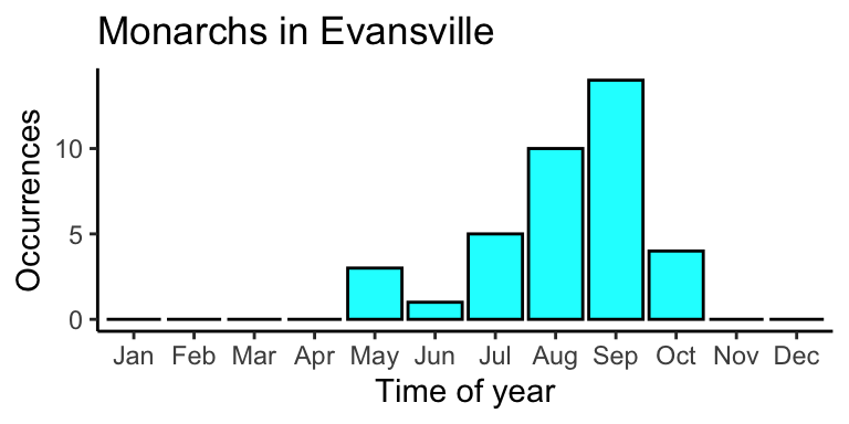
# Get monarch taxonKey
monarch <- name_backbone("Danaus plexippus")$usageKey

# remember to set up your GBIF credentials to use occ_download()
# test <- rgbif::occ_download(pred("taxonKey", monarch),format = "SIMPLE_CSV")

# Evansville and surrounding area
wkt <- "POLYGON((-88.54 38.54, -88.54 37.80, -86.74 37.80, -86.74 38.54, -88.54 38.54))"
EV_monarchs <- occ_count(facet=c("month"), taxonKey=monarch, geometry=wkt)

library(tidyverse)
# Make month columns into integers
EV_monarchs$month <- as.numeric(EV_monarchs$month)
# Fill in missing months with 0 values
for (i in 1:12) {
  if (!(i %in% EV_monarchs$month)) {
    EV_monarchs <- add_row(EV_monarchs, month = i, count = 0)
  }
}

# Order rows by month
EV_monarchs <- arrange(EV_monarchs, month)

# Make column with text month names
EV_monarchs <- mutate(EV_monarchs, Month = month.abb[month])

# Make Month column factors
EV_monarchs$Month <- factor(EV_monarchs$Month, levels = EV_monarchs$Month)

# Plot the data as a barplot with occurrences for each month
library(ggplot2)
ggplot(EV_monarchs, aes(x = Month, y = count)) + # , fill = count
  geom_bar(stat="identity", color="black", fill = "cyan") + 
  xlab("Time of year") + 
  ylab("Occurrences") + 
  ggtitle("Monarchs in Evansville") +
  # scale_fill_gradient(low="cyan", high="cyan") +
  theme_bw() + 
  theme(panel.border = element_blank(), panel.grid.major = element_blank(),
panel.grid.minor = element_blank(), axis.line = element_line(colour = "black")) 

Next, convert this script into a function

• Determine what the parameters will be (variables that you will change)

  • It would be nice to see the same graphs for monarch butterflies from other locations

  • It would be nice to see the same graphs for different species

• Change names are are specific like “EV_monarchs” to something not specific to the location (EV) or species (monarchs) so that the code reads well regardless of what these 2 variables are set to.

• For functions, I generally change library() to require()

  • The only difference is that require won’t re-load a package if it is already loaded

  • This is optional, since library() will still work

  • Remove duplicates so you only load each library once (unless necessary to reload in a different order)

  • For functions like filter() which exist in multiple packages, always call with :: specifying the package

    • Always use dplyr::filter() never filter()

• Improve your comments here as you go to specify what each step is (what each line is doing)

• If your output is a plot, instead of just plotting, return the plot object at the end

  • If you just let it return, it will plot, but you can also save the output to a variable and modify settings later. (In this case, we will do this to change the bar colors for each duplicate plot.)

plot_sightings <- function(species = "Danaus plexippus", location = wkt, title = "Monarchs in Evansville") {
  require(rgbif)
  require(tidyverse)
  
  # Get species taxonKey
  spec_id <- name_backbone(species)$usageKey
  
  # Get data from rgbif for the passed species at the passed location
  sightings <- occ_count(facet=c("month"), taxonKey=spec_id, geometry=location)
  
  library(tidyverse)
  # Make month columns into integers
  sightings$month <- as.numeric(sightings$month)
  # Fill in missing months with 0 values
  for (i in 1:12) {
    if (!(i %in% sightings$month)) {
      sightings <- add_row(sightings, month = i, count = 0)
    }
  }
  
  # Order rows by month
  sightings <- arrange(sightings, month)
  
  # Make column with text month names
  sightings <- mutate(sightings, Month = month.abb[month])
  
  # Make Month column factors
  sightings$Month <- factor(sightings$Month, levels = sightings$Month)
  
  # Plot the data as a barplot with occurrences for each month
  plt <- ggplot(sightings, aes(x = Month, y = count)) + # , fill = count
    geom_bar(stat="identity", color="black", fill = "cyan") + 
    xlab("Time of year") + 
    ylab("Occurrences") + 
    ggtitle(title) +
    theme_bw() + 
    theme(panel.border = element_blank(), panel.grid.major = element_blank(),
  panel.grid.minor = element_blank(), axis.line = element_line(colour = "black")) 
  
  return(plt)
}

Now to run it we can do:

• Note that output plot size is set here for Quarto with {r fig.width=4, fig.height=2} for the code block

• We will have to set this in our Shiny app in a different way later

# Monarch butterfly (Danaus plexippus)
plot_sightings(species = "Danaus plexippus", location = wkt, "Monarchs in Evansville")

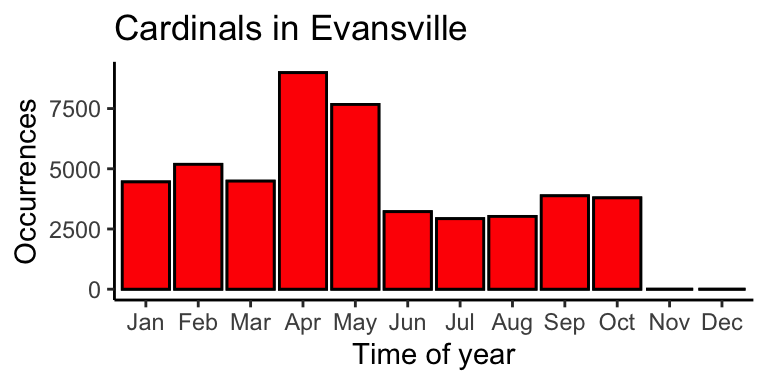
# Northern Cardinal (Cardinalis cardinalis)
plot_sightings(species = "Cardinalis cardinalis", location = wkt, "Cardinals in Evansville") + 
  geom_bar(stat="identity", color="black", fill = "red")

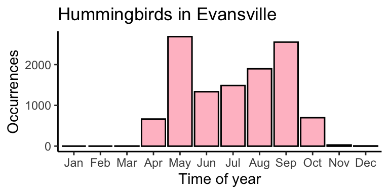
# Ruby Throated Hummingbird (Archilochus colubris)
plot_sightings(species = "Archilochus colubris", location = wkt, "Hummingbirds in Evansville") + 
  geom_bar(stat="identity", color="black", fill = "pink")

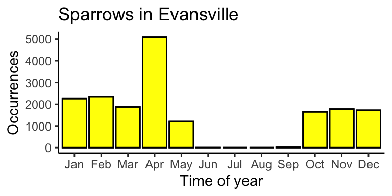
# White-Throated Sparrow (Zonotrichia albicollis)
plot_sightings(species = "Zonotrichia albicollis", location = wkt, "Sparrows in Evansville") + 
  geom_bar(stat="identity", color="black", fill = "yellow")

Helper functions

Sometimes a variable is not simply a single word, number, or boolean. In this case, you may need to define additional functions to create the variable given a simpler input

• location is set with:

# Evansville and surrounding area
wkt <- "POLYGON((-88.54 38.54, -88.54 37.80, -86.74 37.80, -86.74 38.54, -88.54 38.54))"

• These are the four corners of a rectangle as Latitude and Longitude in counterclockwise direction around the rectangle (the direction is important, clockwise will exclude the area inside)

• I defined this manually using the tool here and Apple/Google Maps

  • https://www.gbif.org/occurrence/search?basis_of_record=HUMAN_OBSERVATION&has_coordinate=true&has_geospatial_issue=false&taxon_key=5133088&year=1990,2024&geometry=POLYGON((-88.54438%2037.48459,-86.74461%2037.48459,-86.74461%2038.86468,-88.54438%2038.86468,-88.54438%2037.48459))

• To simplify this, it would be nice to have a function that takes either a single Latitude and Longitude or a city name and generates the wkt output.

library(tidygeocoder)

# Create table of possible cities to check
locs <- tibble::tribble(
~name,            ~address,
"Evansville",     "Evansville, IN",
"West Lafayette", "West Lafayette, IN 47907", 
"Davis",          "Davis, CA",
"Seattle",        "Seattle, WA",
"New Jersey",     "New Jersey, NY",
"Miami",          "Miami, FL",
"LA",             "Los Angelos, CA"
)

# Get latitude and longitude
locs <- geocode(locs, address, method = "osm", lat = latitude, long = longitude)

Passing 7 addresses to the Nominatim single address geocoder

Query completed in: 7.1 seconds

# Create function to generate string with 4 corners for POLYGON call
generate_polygon <- function(lat, long, d_lg=0.9, d_lt=0.37) {
  # "POLYGON((-88.54 38.54, -88.54 37.80, -86.74 37.80, -86.74 38.54, -88.54 38.54))"
  p = paste0("POLYGON((",
             long-d_lg, " ", lat+d_lt, ", ",
             long-d_lg," ", lat-d_lt, ", ",
             long+d_lg," ", lat-d_lt, ", ",
             long+d_lg," ", lat+d_lt, ", ",
             long-d_lg, " ", lat+d_lt,
             "))")
  return(p)
}

# Test function with anu location
anu <- generate_polygon(locs$latitude[1], locs$longitude[1])

# Monarch butterfly (Danaus plexippus) at anu
plot_sightings(species = "Danaus plexippus", location = anu)

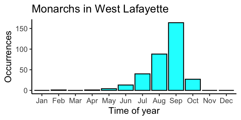
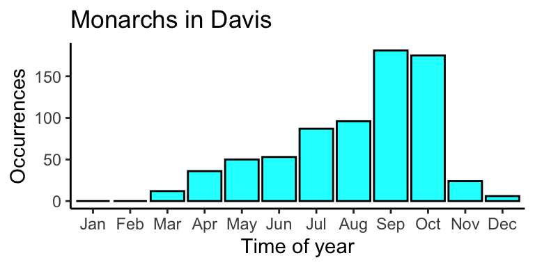
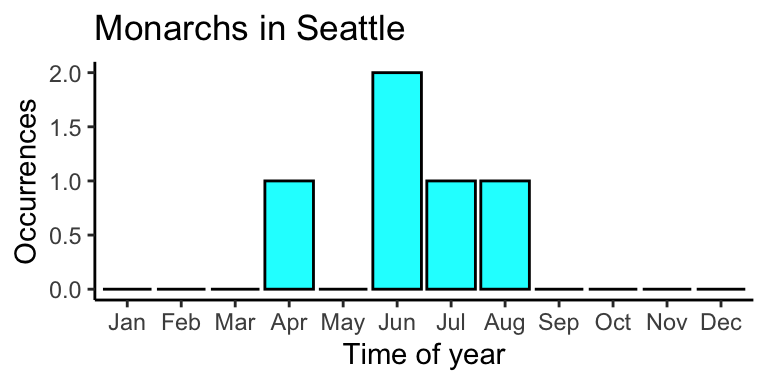
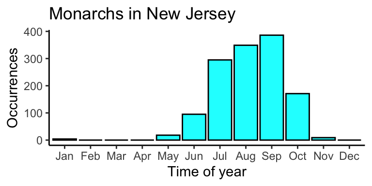
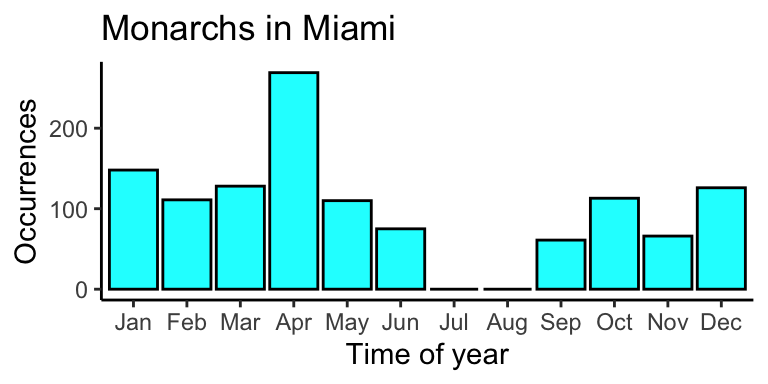
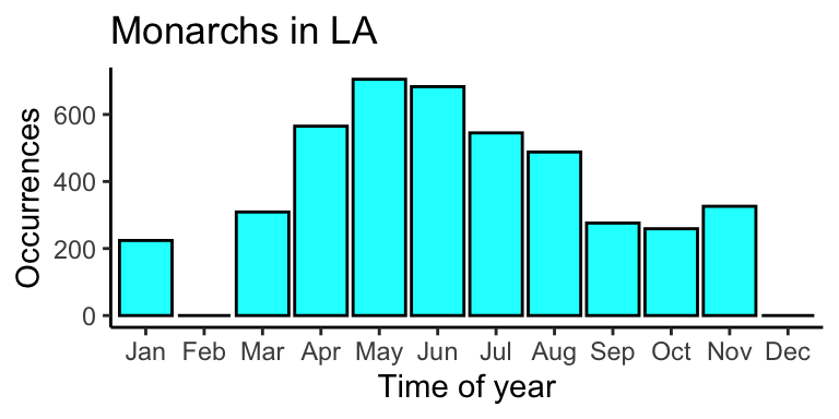
# Populate a column in the data frame with the POLYGON call for each location
locs2 <- mutate(locs, polygon = generate_polygon(locs$latitude, locs$longitude))
## THIS DOESN'T WORK BECAUSE PASTE IS NOT VECTORIZED

# Create function to generate string with 4 corners for POLYGON call
generate_polygon <- function(lat, long, d_lg=0.9, d_lt=0.37) {
  # Paste is not vectorize, use sprintf instead (limit decimals to 4 places)
  p = sprintf("POLYGON((%.4f %.4f, %.4f %.4f, %.4f %.4f, %.4f %.4f, %.4f %.4f))", 
              long-d_lg, lat+d_lt, 
              long-d_lg, lat-d_lt,
              long+d_lg, lat-d_lt,
              long+d_lg, lat+d_lt,
              long-d_lg, lat+d_lt
              )
  return(p)
}

# Populate a column in the data frame with the POLYGON call for each location
locs <- mutate(locs, polygon = generate_polygon(locs$latitude, locs$longitude))
## THIS WORKS NOW

# Plot all locations
for (i in 1:nrow(locs)) {
  plt <- plot_sightings(species = "Danaus plexippus", location = locs$polygon[i], 
                        paste0("Monarchs in ", locs$name[i]))
  print(plt)
}

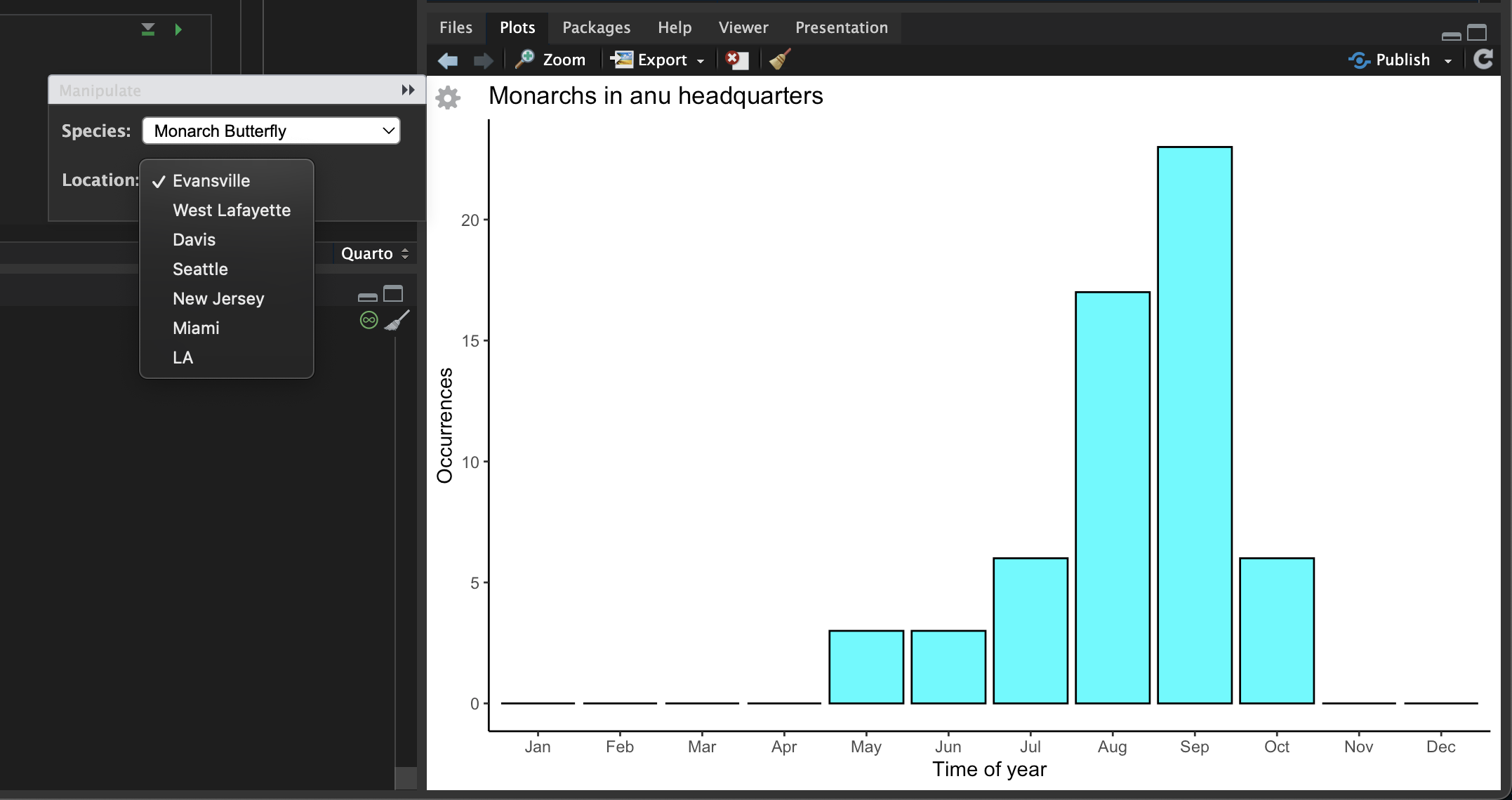
Use manipulate() in RStudio for quick and simple interactive plotting

• The manipulate package only works in RStudio, but it gives you a very quick and simple way to get drop downs and other selectors like you would do in a Shiny app without a lot of coding.

• You can use these sorts of controls:

  • Sliders

  • Dropdown pickers

  • Checkboxes

  • And combinations of the above

  # Very simple example to make sure manipulate is working
  library(manipulate)
  manipulate(plot(1:X), X = slider(1, 10))

• More info here:

  • https://support.posit.co/hc/en-us/articles/200551906-Interactive-Plotting-with-Manipulate-in-the-RStudio-IDE

• A simple example using our dataset and function:

library(manipulate)

manipulate(
  plot_sightings(species = Species, location = locs$polygon[1], 
                        paste0("Monarchs in ", locs$name[1])),
  Species = picker(
    "Monarch Butterfly" = "Danaus plexippus", 
    "Northern Cardinal" = "Cardinalis cardinalis", 
    "Ruby Throated Hummingbird" = "Archilochus colubris",
    "White-Throated Sparrow" = "Zonotrichia albicollis"),
  Location = picker(
    "Evansville" = "Evansville, IN",
    "West Lafayette" = "West Lafayette, IN 47907", 
    "Davis" = "Davis, CA",
    "Seattle" = "Seattle, WA",
    "New Jersey" = "New Jersey, NY",
    "Miami" = "Miami, FL",
    "LA" = "Los Angelos, CA"
  )
)

• You can’t view manipulate in the browser, so I’ll paste a screenshot here and show a live demo during the tutorial:

  

• Another similar package that I haven’t tried based on manipulate is manipulateWidget

  • https://cran.r-project.org/web/packages/manipulateWidget/vignettes/manipulateWidgets.html

Now on to a Shiny app

• A Shiny app gives you more control over the look and feel, more options as far as the ways to interact or display your data, and can run in a web browser locally or across the internet without requiring the viewer to have R or your code running on their system.

Helper function add_polygon_col.R:

###############################################################################
# Sven Nelson                                                                 #
# 6/24/2024                                                                   #
# Function for generating a polygon with 4 corners for RGBIF                  #
###############################################################################

require(tidygeocoder)

# Function to return df with polygon column
add_polygon_col <- function(df) {
  # Create function to generate string with 4 corners for POLYGON call
  generate_polygon <- function(lat, long, d_lg=0.9, d_lt=0.37) {
    # Paste is not vectorize, use sprintf instead (limit decimals to 4 places)
    p = sprintf("POLYGON((%.4f %.4f, %.4f %.4f, %.4f %.4f, %.4f %.4f, %.4f %.4f))", 
                long-d_lg, lat+d_lt, 
                long-d_lg, lat-d_lt,
                long+d_lg, lat-d_lt,
                long+d_lg, lat+d_lt,
                long-d_lg, lat+d_lt
    )
    return(p)
  }
  # Populate a column in the data frame with the POLYGON call for each location
  df <- mutate(df, polygon = generate_polygon(df$latitude, df$longitude))
  return(df)
}

app.R:

###############################################################################
# Sven Nelson                                                                 #
# 6/24/2024                                                                   #
# Shiny app for plotting species occurrence from GBIF.                        #
###############################################################################

#### Imports ####
require(shiny)
require(tidygeocoder)
require(memoise)

source("../R/plot_sightings.R")
source("../R/add_polygon_col.R")

#### Setup ####
# Set up a dataframe to use connecting names with species
specs <- tibble::tribble(
  ~name,                        ~species,                 ~short_name,    ~clr,
  "Monarch Butterfly",          "Danaus plexippus",       "Monarch",      "cyan",
  "Northern Cardinal",          "Cardinalis cardinalis",  "Cardinal",     "red",
  "Ruby Throated Hummingbird",  "Archilochus colubris",   "Hummingbird",  "pink",
  "White-Throated Sparrow",     "Zonotrichia albicollis", "Sparrow",      "yellow"
)

# Create the table of possible cities to check
locs <- tibble::tribble(
  ~name,            ~address,
  "Evansville",     "Evansville, IN",
  "West Lafayette", "West Lafayette, IN 47907", 
  "Davis",          "Davis, CA",
  "Seattle",        "Seattle, WA",
  "New Jersey",     "New Jersey, NY",
  "Miami",          "Miami, FL",
  "LA",             "Los Angelos, CA"
)
# Variable to keep track of whether data needs to be reloaded
reload_data <- TRUE
if (file.exists("locs.rds")) {
  locs2 <- readRDS("locs.rds")
  
  if (dplyr::all_equal(locs, locs2[,1:2]) & ncol(locs2) == 5) {
    locs <- locs2
    reload_data <- FALSE
  }
} 

if (reload_data) {
  # Get latitude and longitude
  locs <- geocode(locs, address, method = "osm", lat = latitude, long = longitude)
  
  # Populate a column in the data frame with the POLYGON call for each location
  locs <- add_polygon_col(locs)
  saveRDS(locs, file = "locs.rds")
}

#### User Interface ####
# Define UI for application that draws a histogram
ui <- fluidPage(

  # Application title
  titlePanel("Organism migration tracking"),

  # Sidebar with a slider input for number of bins 
  sidebarLayout(
    sidebarPanel(
      selectInput("spec_pick", "Organism", choices = specs$name),
      selectInput("loc_pick", "Location", choices = locs$name)
    ),

    # Show a plot of the generated distribution
    mainPanel(
      plotOutput("sightingsPlot", width = 400, height = 200) # Set size here
    )
  )
)

#### Server function ####
# Define server logic required to draw a histogram
server <- function(input, output) {

  output$sightingsPlot <- renderPlot({
    # generate bins based on input$bins from ui.R
    sp_nm <- input$spec_pick
    lc_nm <- input$loc_pick
    sp <- specs[specs$name == sp_nm,]$species
    sp_col <- specs[specs$name == sp_nm,]$clr
    lc <- locs[locs$name == lc_nm,]$polygon
    
    plot_sightings(species = sp, location = lc, paste0(sp_nm, " in ", lc_nm)) + 
      geom_bar(stat="identity", color="black", fill = sp_col)
  })
}

#### Run app ####
shinyApp(ui = ui, server = server)

Shiny Modules

• Convert to module

  • https://shiny.posit.co/r/articles/improve/modules/

  • We will end up with a .R file with the module code, which we can run in a app.R shiny app.

The file sightingsModule.R below:

###############################################################################
# Sven Nelson                                                                 #
# 6/24/2024                                                                   #
# Shiny app module for plotting species occurrence from GBIF.                 #
###############################################################################

#### User Interface ####
# Define UI for application that draws a histogram
sightingsInput <- function(id, label = "Sightings", specs, locs, sel = "Monarch Butterfly") {
  ns <- NS(id)
  tagList(
    h4(label),
    selectInput(ns("spec_pick"), "Organism", choices = specs$name, selected = sel),
    selectInput(ns("loc_pick"), "Location", choices = locs$name)
  )
}

sightingsOutput <- function(id, label = "Sightings") {
  ns <- NS(id)
  tagList(
    plotOutput(ns("sightingsPlot"), width = 400, height = 200)
  )
}

#### Server function ####
# Define server logic required to draw a histogram
sightingsServer <- function(id, specs, locs) {
  moduleServer(
    id,
    function(input, output, session) {
      output$sightingsPlot <- renderPlot({
        # generate bins based on input$bins from ui.R
        sp_nm <- input$spec_pick
        lc_nm <- input$loc_pick
        sp <- specs[specs$name == sp_nm,]$species
        sp_col <- specs[specs$name == sp_nm,]$clr
        lc <- locs[locs$name == lc_nm,]$polygon
        
        plot_sightings(species = sp, location = lc, paste0(sp_nm, " in ", lc_nm)) + 
          geom_bar(stat="identity", color="black", fill = sp_col)
      })
    }
  )
}

The file app.R with the shiny app using a single instance of the same module.

###############################################################################
# Sven Nelson                                                                 #
# 6/24/2024                                                                   #
# Shiny app for plotting species occurrence from GBIF.                        #
###############################################################################

#### Imports ####
require(shiny)
require(tidygeocoder)

source("../R/plot_sightings.R")
source("../R/add_polygon_col.R")
source("../R/sightingsModule.R")

#### Setup ####
# Set up a dataframe to use connecting names with species
specs <- tibble::tribble(
  ~name,                        ~species,                 ~short_name,    ~clr,
  "Monarch Butterfly",          "Danaus plexippus",       "Monarch",      "cyan",
  "Northern Cardinal",          "Cardinalis cardinalis",  "Cardinal",     "red",
  "Ruby Throated Hummingbird",  "Archilochus colubris",   "Hummingbird",  "pink",
  "White-Throated Sparrow",     "Zonotrichia albicollis", "Sparrow",      "yellow"
)

# Create the table of possible cities to check
locs <- tibble::tribble(
  ~name,            ~address,
  "Evansville",     "Evansville, IN",
  "West Lafayette", "West Lafayette, IN 47907", 
  "Davis",          "Davis, CA",
  "Seattle",        "Seattle, WA",
  "New Jersey",     "New Jersey, NY",
  "Miami",          "Miami, FL",
  "LA",             "Los Angelos, CA"
)
# Variable to keep track of whether data needs to be reloaded
reload_data <- TRUE
if (file.exists("locs.rds")) {
  locs2 <- readRDS("locs.rds")
  
  if (dplyr::all_equal(locs, locs2[,1:2]) & ncol(locs2) == 5) {
    locs <- locs2
    reload_data <- FALSE
  }
} 

if (reload_data) {
  # Get latitude and longitude
  locs <- geocode(locs, address, method = "osm", lat = latitude, long = longitude)
  
  # Populate a column in the data frame with the POLYGON call for each location
  locs <- add_polygon_col(locs)
  saveRDS(locs, file = "locs.rds")
}

#### User Interface ####
# Define UI for application that draws a histogram
ui <- fluidPage(
  
  # Application title
  titlePanel("Organism migration tracking"),
  
  # Sidebar with a slider input for number of bins 
  sidebarLayout(
    sidebarPanel(
      sightingsInput("plot1", "Plot 1", specs, locs)
    ),
    
    # Show a plot of the generated distribution
    mainPanel(
      sightingsOutput("plot1", "Plot 1")
    )
  )
)

#### Server function ####
# Define server logic required to draw a histogram
server <- function(input, output) {
  sightingsServer("plot1", specs, locs)
}

#### Run app ####
shinyApp(ui = ui, server = server)

Multiple instances

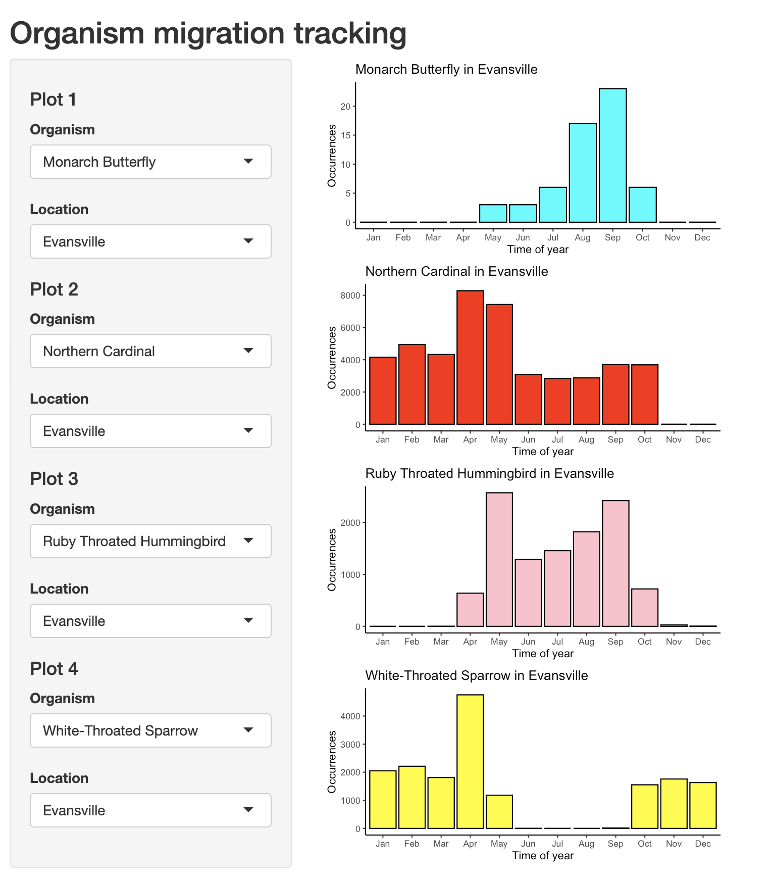
The file app.R with the shiny app using multiple instances of the same module.

###############################################################################
# Sven Nelson                                                                 #
# 6/24/2024                                                                   #
# Shiny app for plotting species occurrence from GBIF.                        #
###############################################################################

#### Imports ####
require(shiny)
require(tidygeocoder)

source("../R/plot_sightings.R")
source("../R/add_polygon_col.R")
source("../R/sightingsModule.R")

#### Setup ####
# Set up a dataframe to use connecting names with species
specs <- tibble::tribble(
  ~name,                        ~species,                 ~short_name,    ~clr,
  "Monarch Butterfly",          "Danaus plexippus",       "Monarch",      "cyan",
  "Northern Cardinal",          "Cardinalis cardinalis",  "Cardinal",     "red",
  "Ruby Throated Hummingbird",  "Archilochus colubris",   "Hummingbird",  "pink",
  "White-Throated Sparrow",     "Zonotrichia albicollis", "Sparrow",      "yellow"
)

# Create the table of possible cities to check
locs <- tibble::tribble(
  ~name,            ~address,
  "Evansville",     "Evansville, IN",
  "West Lafayette", "West Lafayette, IN 47907", 
  "Davis",          "Davis, CA",
  "Seattle",        "Seattle, WA",
  "New Jersey",     "New Jersey, NY",
  "Miami",          "Miami, FL",
  "LA",             "Los Angelos, CA"
)
# Variable to keep track of whether data needs to be reloaded
reload_data <- TRUE
if (file.exists("locs.rds")) {
  locs2 <- readRDS("locs.rds")
  
  if (dplyr::all_equal(locs, locs2[,1:2]) & ncol(locs2) == 5) {
    locs <- locs2
    reload_data <- FALSE
  }
} 

if (reload_data) {
  # Get latitude and longitude
  locs <- geocode(locs, address, method = "osm", lat = latitude, long = longitude)
  
  # Populate a column in the data frame with the POLYGON call for each location
  locs <- add_polygon_col(locs)
  saveRDS(locs, file = "locs.rds")
}

#### User Interface ####
# Define UI for application that draws a histogram
ui <- fluidPage(
  
  # Application title
  titlePanel("Organism migration tracking"),
  
  # Sidebar with a slider input for number of bins 
  sidebarLayout(
    sidebarPanel(
      sightingsInput("plot1", "Plot 1", specs, locs, sel = "Monarch Butterfly"),
      sightingsInput("plot2", "Plot 2", specs, locs, sel = "Northern Cardinal"),
      sightingsInput("plot3", "Plot 3", specs, locs, sel = "Ruby Throated Hummingbird"),
      sightingsInput("plot4", "Plot 4", specs, locs, sel = "White-Throated Sparrow")
    ),
    
    # Show a plot of the generated distribution
    mainPanel(
      sightingsOutput("plot1", "Plot 1"),
      sightingsOutput("plot2", "Plot 2"),
      sightingsOutput("plot3", "Plot 3"),
      sightingsOutput("plot4", "Plot 4")
    )
  )
)

#### Server function ####
# Define server logic required to draw a histogram
server <- function(input, output) {
  sightingsServer("plot1", specs, locs)
  sightingsServer("plot2", specs, locs)
  sightingsServer("plot3", specs, locs)
  sightingsServer("plot4", specs, locs)
}

#### Run app ####
shinyApp(ui = ui, server = server)

Here’s what it looks like:

More Shiny things to try on your own

• Install bslib package and test out additional formatting options including card() for nice cards

  • https://rstudio.github.io/bslib/articles/cards/#shiny

• Convert Shiny code to work in Quarto

  • App complexity is limited to what can run in a browser
  • This has more support for Shiny in python than in R

• Add Caching to your Shiny app for faster loading without re-downloading or re-processing data that hasn’t changed.

  • https://shiny.posit.co/r/articles/improve/caching/